Page 40 - Krész, Miklós, and Andrej Brodnik (eds.). MATCOS-13. Proceedings of the 2013 Mini-Conference on Applied Theoretical Computer Science. Koper: University of Primorska Press, 2016.
P. 40
n on shared memory [1] are discussed. All the constructed ηin+1 = ηin + τ (ag ηin−1 − 2ηin + ηin+1
algorithms provide us with the solutions of the problem that h2
coincide with the experimental data. The special method −
of parallelization on the machines with shared memory was
developed and applied to the constructed algorithms, that − v ηin − ηin−1 − W (ηin, Hin)), i = 1, ..., M. (6)
reduces the computational time greatly not only compared h
to the sequential implementation, but to the classical way
of parallelization with the direct usage of OpenMP pragmas Here M is the number of spatial steps, size of which h is
as well. chosen from the condition:
maxi |TiN (h) − TiN (2h)| < 0.02, (7)
maxi TiN (2h)
2. MATHEMATICAL BASIS where N is the number of time steps. Size of time step
τ must satisfy a stability condition for explicit difference
2.1 Mathematical model schemes, that is theoretically unknown, and is fitted exper-
imentally. The table 1 represents values of K(h) and τ (h)
The simplest one-dimensional FGC model in the enthalpy corresponding to different values of h. Here L = 0.1 is length
formulation includes three equations: of the tube.
∂T = as ∂2T + αs(H − T − Q η), (1) h L · 2−10 L · 2−11 L · 2−12 L · 2−13 L · 2−14
∂t ∂x2 cg τ (h) 2−16 2−17 2−19 2−21 2−23
K(h)
0.159 0.096 0.053 0.028 0.014
∂H = ag ∂2H − v ∂H + αg(T −H + Q η), (2) Table 1: Values of K(h) and τ (h) corresponding to
∂t ∂x2 ∂x cg different values of h
∂η = ag ∂ 2η − v ∂η − W (η, H). (3)
∂t ∂ x2 ∂x
Meanwhile away from the flame front, the solution func-
Here ai = λi/ciρi is the coefficient of thermal diffusivity tions are quite smooth and don’t need such small steps (see
graphic example at Figure 2). Thus, one way to speed up
of the i-th phase, ci, ρi, λi are respectively, specific heat
at constant pressure, density and thermal conductivity of
i-th phase (i = s for porous solid, i = g for gas), αs =
α α
(1−m)cs ρs , αg = mcg ρg , m - porosity, α - interphase heat
transfer rate, v - flow rate of the combustible mixture, T ≡
Ts, cgH = cgTg + Qη is full gas enthalpy, where Ti is the
temperature of the i-th phase, Q is energy release of the re-
action, W (η, H) = k0 η e−E/R(H − Q η) - the chemical reaction
cg
rate according to Arrhenius law, η - relative concentration
of reactive component of the combustible mixture, k0 - pre-
exponential factor, E - activation energy, R - universal gas
constant. It is worth noting here that the speed of the wave
u is a priori unknown.
The Cauchy problem is stated by adding the Dirichlet bound- Figure 2: Graph example of the temperature of solid
T , obtained numerically
ary conditions on the left edge and the Neumann ones on the
the computation seems to be the introduction of an adap-
right. The initial data correspond to the preheated porous tive grid. It should depend on the solution from the previous
time step and be concentrated in the area of the chemical
medium. transformation. It’s carried out as follows. Let there be a
full-length regular coarse spatial grid. Implementation of
2.2 Implementation on a regular and adaptive one time step of the difference scheme on it with the corre-
sponding big time step provides us with the boundary con-
meshes ditions on the next time layer for the small task, that is
stated in the vicinity of the chemical reaction zone similarly
As there is no analytical solution of the problem the suit- the large one. For this enclosed task the denser time-space
ability of all the constructed algorithms is estimated by com- mesh is used. The initial data and boundary conditions at
parison with the solution obtained on the regular fine mesh the every time layer are obtained by the means of linear in-
by using the explicit difference scheme: terpolation from the coarse mesh. After the execution of all
the steps of the subproblem the values of coarse-grid solu-
Tin+1 = Tin + τ (as Tin−1 − 2Tin + Tin+1 + tions in the nodes used for interpolation are replaced with
h2 the corresponding values from the embedded problem (see
Figure 3, where n is the number of the current time layer
+ αs(Hin − Tin − Q ηin )), i = 1, ..., M (4) of the general problem, p is the number of time steps of the
cg subproblem, i0 is the number of the node where W gets its
maximum). The dense grid moves according to the prop-
Hin+1 = Hin + τ (ag Hin−1 − 2Hin + Hin+1 − v Hin − Hin−1 +
h2 h
+ αg (Tin − Hin + Q ηin )), i = 1, ..., M (5)
cg
m a t c o s -1 3 Proceedings of the 2013 Mini-Conference on Applied Theoretical Computer Science 40
Koper, Slovenia, 10-11 October
algorithms provide us with the solutions of the problem that h2
coincide with the experimental data. The special method −
of parallelization on the machines with shared memory was
developed and applied to the constructed algorithms, that − v ηin − ηin−1 − W (ηin, Hin)), i = 1, ..., M. (6)
reduces the computational time greatly not only compared h
to the sequential implementation, but to the classical way
of parallelization with the direct usage of OpenMP pragmas Here M is the number of spatial steps, size of which h is
as well. chosen from the condition:
maxi |TiN (h) − TiN (2h)| < 0.02, (7)
maxi TiN (2h)
2. MATHEMATICAL BASIS where N is the number of time steps. Size of time step
τ must satisfy a stability condition for explicit difference
2.1 Mathematical model schemes, that is theoretically unknown, and is fitted exper-
imentally. The table 1 represents values of K(h) and τ (h)
The simplest one-dimensional FGC model in the enthalpy corresponding to different values of h. Here L = 0.1 is length
formulation includes three equations: of the tube.
∂T = as ∂2T + αs(H − T − Q η), (1) h L · 2−10 L · 2−11 L · 2−12 L · 2−13 L · 2−14
∂t ∂x2 cg τ (h) 2−16 2−17 2−19 2−21 2−23
K(h)
0.159 0.096 0.053 0.028 0.014
∂H = ag ∂2H − v ∂H + αg(T −H + Q η), (2) Table 1: Values of K(h) and τ (h) corresponding to
∂t ∂x2 ∂x cg different values of h
∂η = ag ∂ 2η − v ∂η − W (η, H). (3)
∂t ∂ x2 ∂x
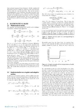
Meanwhile away from the flame front, the solution func-
Here ai = λi/ciρi is the coefficient of thermal diffusivity tions are quite smooth and don’t need such small steps (see
graphic example at Figure 2). Thus, one way to speed up
of the i-th phase, ci, ρi, λi are respectively, specific heat
at constant pressure, density and thermal conductivity of
i-th phase (i = s for porous solid, i = g for gas), αs =
α α
(1−m)cs ρs , αg = mcg ρg , m - porosity, α - interphase heat
transfer rate, v - flow rate of the combustible mixture, T ≡
Ts, cgH = cgTg + Qη is full gas enthalpy, where Ti is the
temperature of the i-th phase, Q is energy release of the re-
action, W (η, H) = k0 η e−E/R(H − Q η) - the chemical reaction
cg
rate according to Arrhenius law, η - relative concentration
of reactive component of the combustible mixture, k0 - pre-
exponential factor, E - activation energy, R - universal gas
constant. It is worth noting here that the speed of the wave
u is a priori unknown.
The Cauchy problem is stated by adding the Dirichlet bound- Figure 2: Graph example of the temperature of solid
T , obtained numerically
ary conditions on the left edge and the Neumann ones on the
the computation seems to be the introduction of an adap-
right. The initial data correspond to the preheated porous tive grid. It should depend on the solution from the previous
time step and be concentrated in the area of the chemical
medium. transformation. It’s carried out as follows. Let there be a
full-length regular coarse spatial grid. Implementation of
2.2 Implementation on a regular and adaptive one time step of the difference scheme on it with the corre-
sponding big time step provides us with the boundary con-
meshes ditions on the next time layer for the small task, that is
stated in the vicinity of the chemical reaction zone similarly
As there is no analytical solution of the problem the suit- the large one. For this enclosed task the denser time-space
ability of all the constructed algorithms is estimated by com- mesh is used. The initial data and boundary conditions at
parison with the solution obtained on the regular fine mesh the every time layer are obtained by the means of linear in-
by using the explicit difference scheme: terpolation from the coarse mesh. After the execution of all
the steps of the subproblem the values of coarse-grid solu-
Tin+1 = Tin + τ (as Tin−1 − 2Tin + Tin+1 + tions in the nodes used for interpolation are replaced with
h2 the corresponding values from the embedded problem (see
Figure 3, where n is the number of the current time layer
+ αs(Hin − Tin − Q ηin )), i = 1, ..., M (4) of the general problem, p is the number of time steps of the
cg subproblem, i0 is the number of the node where W gets its
maximum). The dense grid moves according to the prop-
Hin+1 = Hin + τ (ag Hin−1 − 2Hin + Hin+1 − v Hin − Hin−1 +
h2 h
+ αg (Tin − Hin + Q ηin )), i = 1, ..., M (5)
cg
m a t c o s -1 3 Proceedings of the 2013 Mini-Conference on Applied Theoretical Computer Science 40
Koper, Slovenia, 10-11 October