Page 36 - Fister jr., Iztok, and Andrej Brodnik (eds.). StuCoSReC. Proceedings of the 2018 5th Student Computer Science Research Conference. Koper: University of Primorska Press, 2018
P. 36
inition 5. A rule R satisfies Constraint_Itemsets if its contained in a given transaction t. All the missing details of the
antecedent (itemset) contains at least one itemset in Apriori algorithm can be found in [1] and [2].
Constraint_Itemsets.
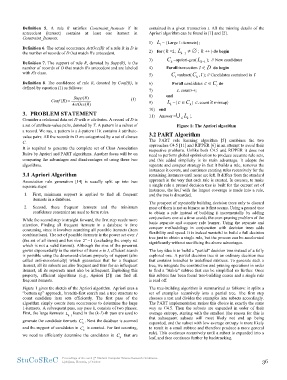
1) L1 = {Large 1-itemsets};
Definition 6. The actual occurrence ActOcc(R) of a rule R in D is
the number of records of D that match R's antecedent. 2) for ( k =2; Lk1 ; k ++ ) do begin
Definition 7. The support of rule R, denoted by Supp(R), is the 3) Ck =apriori-gen( Lk 1 ); // New candidates
number of records of D that match R's antecedent and are labeled 4) Forall transaction t D do begin
with R's class. 5) Ct =subset( Ck , t ); // Candidates contained in t
Definition 8. The confidence of rule R, denoted by Conf(R), is 6) Forall candidates c Ct do
defined by equation (1) as follows: 7) c. count++;
Conf (R) Supp(R) (1) 8) end
ActOcc(R)
9) Lk ={ c Ck | c. count minsup}
3. PROBLEM STATEMENT
10) end
Consider a relational data set D with n attributes. A record of D is
a set of attribute-value pairs, denoted by T. A pattern is a subset of 11) Answer =⋃ k Lk ;
a record. We say, a pattern is a k-pattern if it contains k attribute-
value pairs. All the records in D are categorized by a set of classes Figure 1: The Apriori algorithm
C.
It is required to generate the complete set of Class Association 3.2 PART Algorithm
Rules by Apriori and PART algorithms. Another focus will be on
comparing the advantages and disadvantages of using these two The PART rule learning algorithm [5] combines the two
algorithms. approaches C4.5 [11] and RIPPER [6] in an attempt to avoid their
respective problems. Unlike both C4.5 and RIPPER it does not
3.1 Apriori Algorithm need to perform global optimization to produce accurate rule sets,
and this added simplicity is its main advantage. It adopts the
Association rule generation [14] is usually split up into two separate and conquer strategy in that it builds a rule, removes the
separate steps: instances it covers, and continues creating rules recursively for the
remaining instances until none are left. It differs from the standard
1. First, minimum support is applied to find all frequent approach in the way that each rule is created. In essence, to make
itemsets in a database. a single rule a pruned decision tree is built for the current set of
instances, the leaf with the largest coverage is made into a rule,
2. Second, these frequent itemsets and the minimum and the tree is discarded.
confidence constraint are used to form rules.
The prospect of repeatedly building decision trees only to discard
While the second step is straight forward, the first step needs more most of them is not as bizarre as it first seems. Using a pruned tree
attention. Finding all frequent itemsets in a database is time to obtain a rule instead of building it incrementally by adding
consuming since it involves searching all possible itemsets (item conjunctions one at a time avoids the over-pruning problem of the
combinations). The set of possible itemsets is the power set over I basic separate and conquer rule learner. Using the separate and
(the set of all items) and has size 2n 1 (excluding the empty set conquer methodology in conjunction with decision trees adds
which is not a valid itemset). Although the size of the powerset flexibility and speed. It is indeed wasteful to build a full decision
grows exponentially in the number of items n in I, efficient search tree just to obtain a single rule, but the process can be accelerated
is possible using the downward-closure property of support (also significantly without sacrificing the above advantages.
called anti-monotonicity) which guarantees that for a frequent
itemset, all its subsets are also frequent and thus for an infrequent The key idea is to build a “partial” decision tree instead of a fully
itemset, all its supersets must also be infrequent. Exploiting this explored one. A partial decision tree is an ordinary decision tree
property, efficient algorithms (e.g., Apriori [2]) can find all that contains branches to undefined subtrees. To generate such a
frequent itemsets. tree, we integrate the construction and pruning operations in order
to find a “stable” subtree that can be simplified no further. Once
Figure 1 gives the sketch of the Apriori algorithm. Apriori uses a this subtree has been found tree-building ceases and a single rule
“bottom up” approach, breadth-first search and a tree structure to is read off.
count candidate item sets efficiently. The first pass of the
algorithm simply counts item occurrences to determine the large The tree-building algorithm is summarized as follows: it splits a
1-itemsets. A subsequent pass, say pass k, consists of two phases. set of examples recursively into a partial tree. The first step
First, the large itemsets Lk1 found in the (k-1)-th pass are used to chooses a test and divides the examples into subsets accordingly.
The PART implementation makes this choice in exactly the same
generate the candidate itemsets Ck . Next the database is scanned way as C4.5. Then the subsets are expanded in order of their
average entropy, starting with the smallest (the reason for this is
and the support of candidates in Ck is counted. For fast counting, that subsequent subsets will most likely not end up being
expanded, and the subset with low average entropy is more likely
we need to efficiently determine the candidates in Ck that are to result in a small subtree and therefore produce a more general
rule). This continues recursively until a subset is expanded into a
leaf, and then continues further by backtracking.
StuCoSReC Proceedings of the 2018 5th Student Computer Science Research Conference 36
Ljubljana, Slovenia, 9 October
antecedent (itemset) contains at least one itemset in Apriori algorithm can be found in [1] and [2].
Constraint_Itemsets.
1) L1 = {Large 1-itemsets};
Definition 6. The actual occurrence ActOcc(R) of a rule R in D is
the number of records of D that match R's antecedent. 2) for ( k =2; Lk1 ; k ++ ) do begin
Definition 7. The support of rule R, denoted by Supp(R), is the 3) Ck =apriori-gen( Lk 1 ); // New candidates
number of records of D that match R's antecedent and are labeled 4) Forall transaction t D do begin
with R's class. 5) Ct =subset( Ck , t ); // Candidates contained in t
Definition 8. The confidence of rule R, denoted by Conf(R), is 6) Forall candidates c Ct do
defined by equation (1) as follows: 7) c. count++;
Conf (R) Supp(R) (1) 8) end
ActOcc(R)
9) Lk ={ c Ck | c. count minsup}
3. PROBLEM STATEMENT
10) end
Consider a relational data set D with n attributes. A record of D is
a set of attribute-value pairs, denoted by T. A pattern is a subset of 11) Answer =⋃ k Lk ;
a record. We say, a pattern is a k-pattern if it contains k attribute-
value pairs. All the records in D are categorized by a set of classes Figure 1: The Apriori algorithm
C.
It is required to generate the complete set of Class Association 3.2 PART Algorithm
Rules by Apriori and PART algorithms. Another focus will be on
comparing the advantages and disadvantages of using these two The PART rule learning algorithm [5] combines the two
algorithms. approaches C4.5 [11] and RIPPER [6] in an attempt to avoid their
respective problems. Unlike both C4.5 and RIPPER it does not
3.1 Apriori Algorithm need to perform global optimization to produce accurate rule sets,
and this added simplicity is its main advantage. It adopts the
Association rule generation [14] is usually split up into two separate and conquer strategy in that it builds a rule, removes the
separate steps: instances it covers, and continues creating rules recursively for the
remaining instances until none are left. It differs from the standard
1. First, minimum support is applied to find all frequent approach in the way that each rule is created. In essence, to make
itemsets in a database. a single rule a pruned decision tree is built for the current set of
instances, the leaf with the largest coverage is made into a rule,
2. Second, these frequent itemsets and the minimum and the tree is discarded.
confidence constraint are used to form rules.
The prospect of repeatedly building decision trees only to discard
While the second step is straight forward, the first step needs more most of them is not as bizarre as it first seems. Using a pruned tree
attention. Finding all frequent itemsets in a database is time to obtain a rule instead of building it incrementally by adding
consuming since it involves searching all possible itemsets (item conjunctions one at a time avoids the over-pruning problem of the
combinations). The set of possible itemsets is the power set over I basic separate and conquer rule learner. Using the separate and
(the set of all items) and has size 2n 1 (excluding the empty set conquer methodology in conjunction with decision trees adds
which is not a valid itemset). Although the size of the powerset flexibility and speed. It is indeed wasteful to build a full decision
grows exponentially in the number of items n in I, efficient search tree just to obtain a single rule, but the process can be accelerated
is possible using the downward-closure property of support (also significantly without sacrificing the above advantages.
called anti-monotonicity) which guarantees that for a frequent
itemset, all its subsets are also frequent and thus for an infrequent The key idea is to build a “partial” decision tree instead of a fully
itemset, all its supersets must also be infrequent. Exploiting this explored one. A partial decision tree is an ordinary decision tree
property, efficient algorithms (e.g., Apriori [2]) can find all that contains branches to undefined subtrees. To generate such a
frequent itemsets. tree, we integrate the construction and pruning operations in order
to find a “stable” subtree that can be simplified no further. Once
Figure 1 gives the sketch of the Apriori algorithm. Apriori uses a this subtree has been found tree-building ceases and a single rule
“bottom up” approach, breadth-first search and a tree structure to is read off.
count candidate item sets efficiently. The first pass of the
algorithm simply counts item occurrences to determine the large The tree-building algorithm is summarized as follows: it splits a
1-itemsets. A subsequent pass, say pass k, consists of two phases. set of examples recursively into a partial tree. The first step
First, the large itemsets Lk1 found in the (k-1)-th pass are used to chooses a test and divides the examples into subsets accordingly.
The PART implementation makes this choice in exactly the same
generate the candidate itemsets Ck . Next the database is scanned way as C4.5. Then the subsets are expanded in order of their
average entropy, starting with the smallest (the reason for this is
and the support of candidates in Ck is counted. For fast counting, that subsequent subsets will most likely not end up being
expanded, and the subset with low average entropy is more likely
we need to efficiently determine the candidates in Ck that are to result in a small subtree and therefore produce a more general
rule). This continues recursively until a subset is expanded into a
leaf, and then continues further by backtracking.
StuCoSReC Proceedings of the 2018 5th Student Computer Science Research Conference 36
Ljubljana, Slovenia, 9 October