Page 54 - Fister jr., Iztok, and Andrej Brodnik (eds.). StuCoSReC. Proceedings of the 2016 3rd Student Computer Science Research Conference. Koper: University of Primorska Press, 2016
P. 54
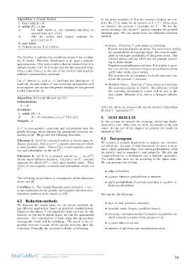
orithm 1 Greedy Method In the given iteration, if X is the current solution, we con-
1: Start with A = ∅. sider the f ∗(v) value for all elemets of X ∈ V ∗. From these
2: while |A| ≤ k do we consider the greatest r elements, set V ˜. We use the
3: For each vertex x, use repeated sampling to greedy strategy only on set V ˜ and we consider the greatest
marginal gain. We can choose from two different reduction
approximate g(A ∪ {x}) method:
4: Add the vertex with largest estimate for
• Degree: Function f ∗ gets values as following:
g(A ∪ {x}) to A. Positive maximalization problem: For each vertex, adding
5: end while the probabilities of outgoing edges. The sum is multi-
6: Output the set A of vertices. plied by the input probability of the given vertex. The
method selects vertices which are the greatest accord-
The function σ satisfies the conditions above if we consider ing to these values.
the IC model. Therefore Nemhauser et al. gave a suitable Negative maximalization problem: It is similar to posi-
approximation. Our main result is that we showed that it is tive one, but the product of values are subtracted from
suitable for the GIC. So it is also true for the expected value uplift value of the given vertex.
σ(wp,v) and σ(wn,v) in the case of the positive and negative The process sets up a sequence for both cases and con-
influence maximization problems. siders the greatest r elements.
Let σ∗ denote σp and σn to facilitate the description of • Modified Degree: Function f ∗ gets values as following:
methods. As seen before σ∗ are monotone, submodular and The process is similar to Degree. The difference is that
non-negative, we can use the greedy strategy for the general the currently investegated vertex will be not in the
model (Algorithm 2) next phase. Because of it, this is a dynamic calcula-
tion.
Algorithm 2 Greedy Method for GIC
Initialization: After the above is executed the greedy method (Algorithm
2) with V ˜ instead of V ∗.
A := ∅
Iteration: 5. TEST RESULTS
1: while |A| ≤ k
2: A = A ∪ arg maxx∈V ∗\A σ∗(A ∪ {x}) In this section we present the program, which was imple-
Output: A mented for test. After that we show the details of the test
cases. At the end of the chapter we present the result for
If σ∗ is non-negative, monotone and submodular then the analysis of GIC.
greedy strategy above ensures the guaranteed accuracy ac-
cording to [8]. We proved the following theorems: 5.1 Test program
Theorem 2. Let G be a network and let w denote input in- We created a scalable framework to analyze our theoreti-
fluence function. Pick a set V ∗ contains elements for which cal solutions. As part of this framework we have a simu-
w gives positive value. Then σpG(w) is non-negative, mono- lator, which generates edge- and vertex-probabilities, what
ton and submodular on the set V ∗. we usually need to measure in real networks. We also use
σ-approximations, a simulation and a heuristic generator.
Theorem 3. Let G be a network and let wn = (w, wup) The uplift value were set up according to the input value.
denote input influence function. Let pick a set V ∗ contains We can generate the follows:
elements for which wup < w(v) gives positive value. Then
σnG(w) is non-negative, monoton and submodular on the set • edge probability
V ∗.
• a priori infection probabilities of vertices
The following proprosition is consequence of the theorems
above and [8]. • uplift probabilities of vertices according to a priori in-
fection probabilities
Corollary 1. The Greedy Heuristic gives at least (1 − 1/e −
)-aprroximation for the positive and negative infection max- We can set the following:
imization problems if the model is GID.
• type of task (positive, negative)
4.2 Reduction methods
• heuristic mode (degree, modified degree)
We decrease the search space for the greedy methods us-
ing different approaches based on practical considerations. • iteration, evaluation method (complete simulation, an-
Based on the above, if the algorithm does not look for the alytic formula heuristic [with parameter t])
solution on the whole search space, we lose the guaranteed
precision. Our expectation is that using the appropriate • a priori infected set size
strategy the result will be satisfying. The speed of the al-
gorithm increase because of the greedy property after the • number of infection and evaluation iteration
reduction. Formally, the methods look like as following:
StuCoSReC Proceedings of the 2016 3rd Student Computer Science Research Conference 54
Ljubljana, Slovenia, 12 October