Page 54 - Fister jr., Iztok, and Andrej Brodnik (eds.). StuCoSReC. Proceedings of the 2018 5th Student Computer Science Research Conference. Koper: University of Primorska Press, 2018
P. 54
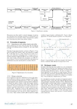
ure 1: Classification pipeline
Histograms are often used in natural language processing number of approximation coefficients [17]. Figure 3 shows
and computer vision problems, because local informations of application of discrete wavelet transform on a time series.
observed object are presented. Those characteristics justify
use of histograms as time series feature vectors. Figure 3: Approximation coefficients of applied db3 discrete
wavelet transform with different decomposition levels
2.1 Extraction of segments
2.1.1 Segmentation with sliding window algorithm 2.2 Dictionary words
Both training and test time series are split into overlapping K-means clustering has been applied on a set of segments
segments with sliding window of length Wc and step length feature vectors, extracted from training time series in previ-
tc < Wc. ous step. Result of clustering is K number of clusters with
centroids being dictionary words. In terms of speed, K-
Example of segments extraction is shown on Figure 2. Time means algorithm is not suitable for large datasets. Because
series of length 3072 values is split onto segments of length of the latter fact, alternative algorithm Mini Batch K-means,
Wc = 256 with step tc = 192. Segments are shown in or- was used. Algorithm uses subset of the dataset per iteration
ange color with grey overlapping parts. In most cases, in- and, consequently, less computations are needed.
dividual segment’s length should not exceed 10% of average For visualization purposes, conversion of segments multidi-
time series length, although this percantage can differ be- mensional feature vectors into three dimensional was done,
tween datasets. Selected window length has a big impact on using principal component analysis (PCA). Mathematical
classification accuracy and should be carefully selected. transformation converts large number of potentially depen-
dant variables to fewer independant variables – principal
Figure 2: Segmentation of a time series components, which hold the most information. Applying
principal component analysis is one of the first steps in anal-
2.1.2 Feature extraction ysis of large, multivariate datasets [13]. Result of clustering
PCA output is visible on Figure 4 with individual cluster
Every segment is described with features being approxima- being presented in unique color and have a centroid marked
tion coefficients of discrete wavelet transform (DWT) func- with a black dot.
tion for a selected decomposition level. With every increase
of decomposition level, number of approximation coefficients
is reduced by nearly a factor of two, but enough informa-
tion is preserved to reconstruct original data. With selected
transform, frequency informations at lower frequencies are
analyzed and time informations in higher frequencies are
gathered [17]. Additional benefit of the transform is data
noise reduction. Db3 discrete wavelet transform function at
first decomposition level was used to define segment’s fea-
ture vector. That results in almost half of segment’s length
StuCoSReC Proceedings of the 2018 5th Student Computer Science Research Conference 56
Ljubljana, Slovenia, 9 October